Sensitivity, uncertainty and calibration
Which parameters matter, how much a result spreads when they are uncertain, which values
make the model match a measurement, and which value hits a design target: the
workbench's Analysis mode and four daedalus commands answer these on any model,
with no scripting.
| Question | Command | Analysis tab |
|---|---|---|
| Which parameters drive this output, and when? | sensitivity |
Sensitivity |
| How much does the result spread? Which inputs cause the spread? | montecarlo, gsa |
Uncertainty |
| Which parameter values fit my measurements? | calibrate |
Calibrate |
| Which value meets my target? | optimize |
Optimize |
Only free parameters can be varied: public parameters with a literal value, the ones that are editable in the variable browser. Parameters computed from others, protected ones and those evaluated at translation give an error that lists the free ones.
In the workbench
Simulate a model, switch to Analysis in the toolbar and tick the parameters to vary. Each tab has its own settings and Run; a progress bar shows while it runs and Cancel stops it.
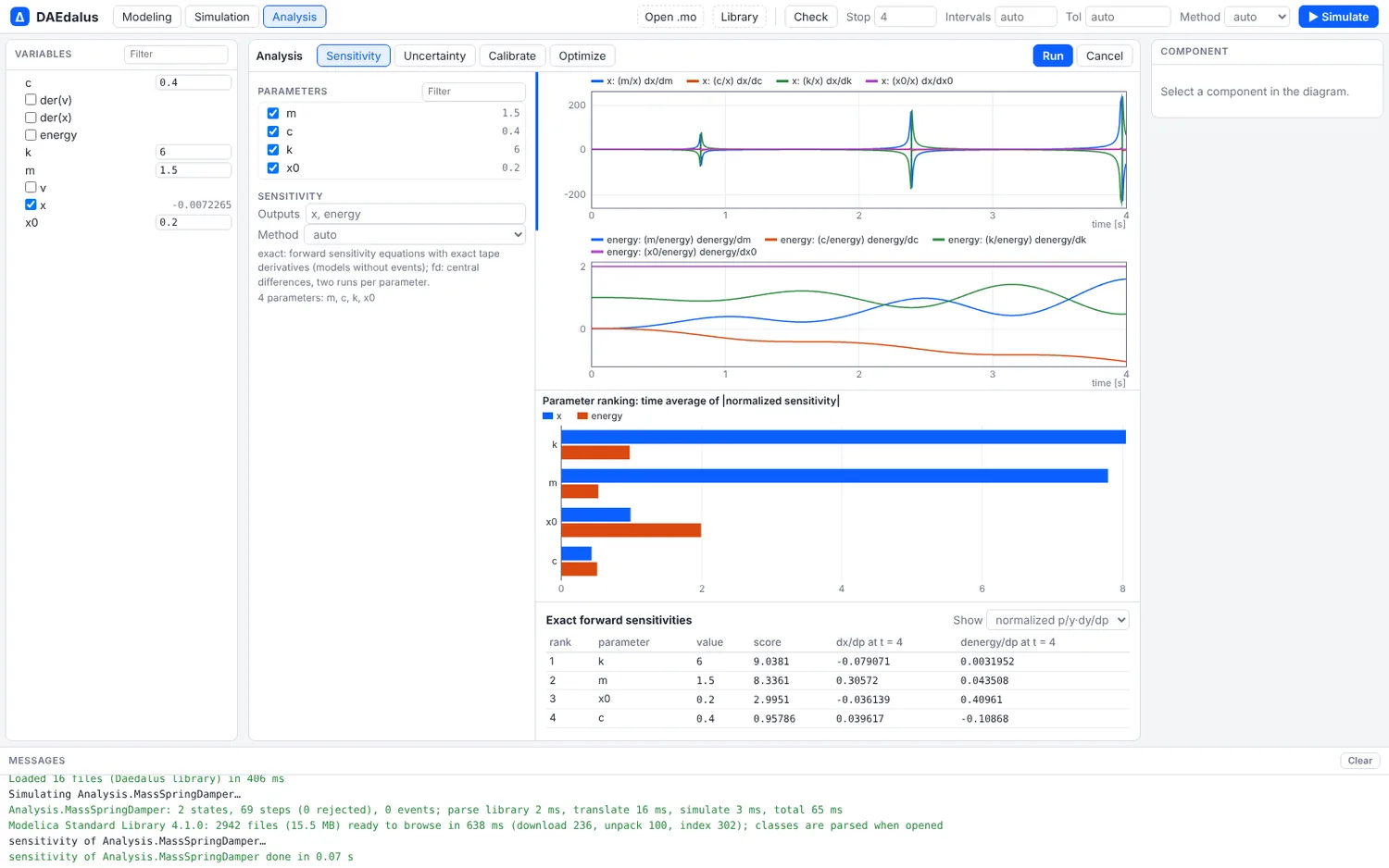
dy/dp over time for each parameter, and a ranking by the time average of the normalized sensitivity.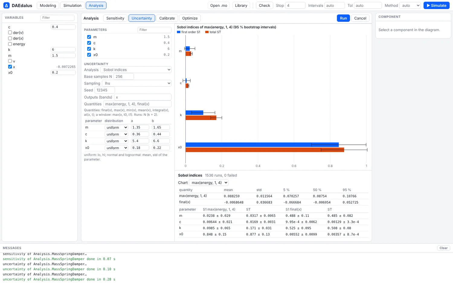
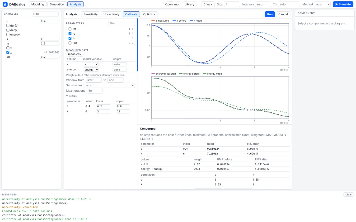
The Calibrate tab loads a CSV, maps its columns to model variables and sets the bounds of each tuner. It plots the measured data against the model before and after the fit, lists the fitted values with standard errors and correlations, and Copy as modifier gives the result as a Modelica modification.
Sensitivity
daedalus sensitivity library/Daedalus -m Daedalus.Examples.QuarterCar.BumpComparison \
    --params linear.m_body,linear.c_spring,linear.c_tyre,bump.h --outputs linear.a_body
sensitivities of Daedalus.Examples.QuarterCar.BumpComparison (central finite differences), 2001 points from t = 0 to 2
note: finite differences used because the exact method failed: step size too small at t = 0.008507344142682349
note: central differences, relative step 1e-4, tolerance 1e-8
ranking (time average of |p/y dy/dp|, summed over outputs):
1. linear.m_body 2.60687e0 (p = 400)
2. linear.c_spring 1.74834e0 (p = 30000)
3. bump.h 1.20919e0 (p = 0.05)
4. linear.c_tyre 5.00763e-1 (p = 250000)--sens-method chooses how:
exactintegrates the forward sensitivity equationsds/dt = df/dx s + df/dpnext to the state, with exact tangents of the compiled model, algebraic loops included. It needs a model withoutwhenclauses anddelay(), and a run without events.fduses two runs per parameter with a relative step of 1e-4 at a tightened tolerance.auto(the default) usesexactwhere it applies and otherwise says why it usedfd, as above, where the hydraulic damper's fast start stops the exact method.
The output holds the time series of dy/dp and of the normalized p/y dy/dp, and -o
writes them as JSON or CSV.
Uncertainty and global sensitivity
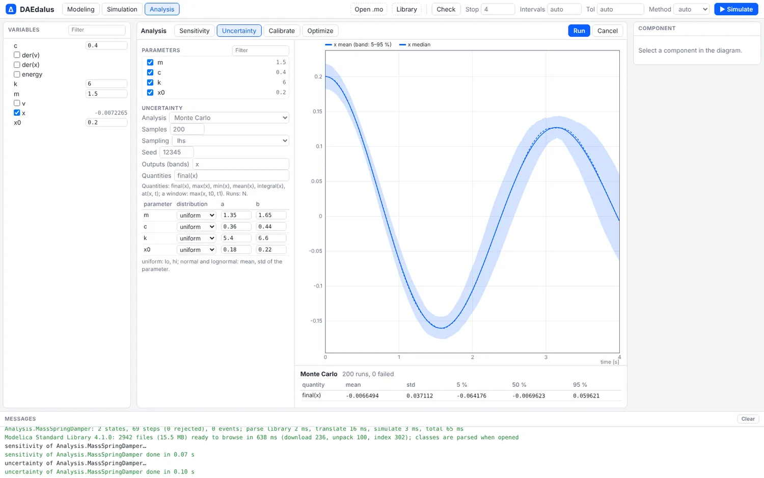
montecarlo samples the parameters from their distributions and reports the mean,
standard deviation and the 5, 50 and 95 % bands of each output; gsa adds Sobol indices
(first-order and total, in N (k + 2) runs) or Morris screening (--morris). Runs use all
cores.
daedalus gsa library/Daedalus -m Daedalus.Examples.QuarterCar.BumpComparison \
    --dist linear.m_body=250:350 --dist linear.c_spring=20e3:40e3 --dist bump.h=normal:0.05:0.01 \
    --qoi 'max(linear.a_body)' -N 128
Sobol indices of Daedalus.Examples.QuarterCar.BumpComparison: 640 runs, 0 failed
quantity mean std 5% 50% 95%
max(linear.a_body) 1.64112e1 3.72167e0 1.04179e1 1.62511e1 2.29829e1
max(linear.a_body) (mean 1.64266e1, variance 1.45367e1):
parameter S1 ST
linear.m_body 0.1981 +-0.088 0.1619 +-0.046
linear.c_spring 0.0079 +-0.028 0.0111 +-0.003
bump.h 0.6979 +-0.191 0.6082 +-0.129The bump height explains about 70 % of the spread in peak body acceleration and the spring rate almost none. That took 14.5 s for 640 runs on four cores.
- Distributions:
p=lo:hi(uniform),p=normal:MEAN:STD,p=lognormal:MEAN:STD; Latin hypercube or random sampling (--sampling), seeded (--seed). - Quantities:
final(x),max(x),min(x),mean(x),integral(x)andat(x,T), each with an optional window such asmax(x,T0,T1).
Calibration
calibrate fits parameters to measured data with a projected Levenberg–Marquardt method.
The CSV has a time column and measured columns, matched to variables by name or with
--map column=var. Here the measurement is a simulated run with m_body = 360 and
c_spring = 36000 plus noise, and the fit starts from the model's 400 and 30000:
daedalus calibrate library/Daedalus -m Daedalus.Examples.QuarterCar.BumpComparison \
    --data meas.csv --tune linear.m_body=250:500 --tune linear.c_spring=15e3:50e3
calibration of Daedalus.Examples.QuarterCar.BumpComparison: 4 iterations, 230 residuals, sensitivities: finite differences
converged: no step reduces the cost further (local minimum)
weighted residual RMS: 3.307286e-1 -> 8.723941e-2
parameter initial fitted std. error
linear.m_body 4.0000000e2 3.5971769e2 2.361e0
linear.c_spring 3.0000000e4 3.5999803e4 3.545e2
correlation:
[ 1.000 0.843]
[ 0.843 1.000]
modifier: (linear(m_body = 359.71769, c_spring = 35999.803))Weights default to one over each column's standard deviation (--weight changes them),
and --window T0:T1 restricts the fit in time.
Optimization
optimize runs Nelder–Mead inside the bounds. The objective is the sum of
--minimize q, --maximize q and --target q=v terms, with the same quantities as
above. Which body mass brings the peak body acceleration over the bump down to 10 m/s²?
daedalus optimize library/Daedalus -m Daedalus.Examples.QuarterCar.BumpComparison \
    --tune linear.m_body=250:600 --target 'max(linear.a_body)=10'
optimization of Daedalus.Examples.QuarterCar.BumpComparison (Nelder-Mead): 29 iterations, 58 runs; simplex converged
objective: 5.751422e0 -> 1.186965e-17
max(linear.a_body): 1.239821e1 -> 1.000000e1
parameter initial optimal
linear.m_body 4.0000000e2 5.0070892e2
modifier: (linear(m_body = 500.70892))Dynamic optimization, where the inputs vary over time and constraints apply along the trajectory, is the job of the CasADi export.
Checked against known answers
crates/daedalus-core/tests/analysis.rs compares these analyses with analytic results:
exponential decay, a mass-spring-damper, the Ishigami function's Sobol indices, Monte
Carlo moments, and parameter recovery from synthetic data.