Solvers
DAEdalus integrates the state-space form der(x) = f(t, x) that the symbolic
backend produces. All methods share the event handling (zero crossings located
on the dense output, event iteration, reinit), the output grid and the
statistics.
| Method | --method |
Kind | Use it for |
|---|---|---|---|
| BDF | bdf (default) |
stiff, multistep, order 1–5 | most models; the role Dassl plays in Dymola |
| Radau IIA | radau |
stiff, implicit Runge–Kutta, order 5 | very stiff or oscillatory problems at tight tolerances; few steps |
| ESDIRK | esdirk |
stiff, diagonally implicit Runge–Kutta, order 4 | stiff models with frequent events (cheap restarts) |
| Auto | auto |
Dopri5 ⇄ BDF | models that are stiff only part of the time (like Lsodar) |
| Dopri5 | dopri5 |
explicit, order 5(4) | non-stiff models |
| RK4, Euler | rk4, euler |
explicit, fixed step | real-time style runs (step = output interval or --step) |
daedalus simulate model.mo -m M --method radau           # pick a method
daedalus simulate model.mo -m M --method bdf --jacobian fd   # finite-difference Jacobian
daedalus test-library lib -m Pkg --method auto # sweep with one methodPer-model choice
The experiment annotation selects the method when --method is not given.
__Dymola_Algorithm (or __Daedalus_Algorithm) maps to the closest method:
| Annotation | Method |
|---|---|
Dassl, Cvode, Ida, Lsode |
bdf |
Lsodar, Lsoda |
auto |
Radau |
radau |
Esdirk23a, Esdirk34a, Esdirk45a, Sdirk34hw |
esdirk |
Dopri45, Dopri853, Cerk* |
dopri5 |
Rkfix2, Rkfix3, Rkfix4 |
rk4 |
Euler |
euler |
State Jacobian
The implicit methods (BDF, Radau, ESDIRK, and BDF inside Auto) need
J = df/dx. Columns that share no row are grouped by a greedy coloring of the
dependency pattern, so one pass gives a whole group.
- Exact (default). Each pass is a forward-mode (tangent) run of the compiled
tape, seeded with the states of one color group, the same machinery as
linearize. Algebraic loops are differentiated implicitly with their symbolic Jacobians. There is no truncation error and no step-size choice. If a column comes out non-finite, that evaluation falls back to differences. - Forward differences (
--jacobian fd,SimOptions::jacobian = Fd): one right-hand-side evaluation per color group. This reproduces the BDF step sequence of earlier versions.
Both cost one pass per color. A tangent pass costs about one to two
right-hand-side evaluations, so the exact Jacobian is about as cheap as the
differences, and its columns are accurate to rounding. The statistics count
tangent passes separately (tangent_evals).
Up to 48 states the iteration matrices are dense; beyond that they use the
sparse LU with a minimum-degree ordering. Radau's complex system
((α + iβ)/h) I - J is solved as the real 2n × 2n system with the real and
imaginary part of each unknown next to each other, which keeps the sparsity.
Radau IIA
src/solver_radau.rs follows Hairer & Wanner's RADAU5 (Solving ODEs II,
IV.8): three Radau IIA stages (order 5, L-stable, stiffly accurate).
- Simplified Newton in transformed variables: one real factorization of
(γ/h) I - Jand one complex one per step size, instead of a3n × 3nsystem. The Jacobian is kept while Newton contracts faster than 0.01; the factorizations are kept while the step size changes by less than 20 %. - Starting values from the collocation polynomial of the last step.
- Embedded error estimate filtered by
((γ/h) I - J)^-1; predictive (Gustafsson) step-size control. Tolerances are mapped as RADAU5 does (0.1 rtol^(2/3)). - Dense output: the collocation polynomial.
ESDIRK
src/solver_esdirk.rs is ESDIRK4(3)6L[2]SA of Kennedy & Carpenter: six stages,
an explicit first stage, diagonal γ = 1/4, L-stable and stiffly accurate,
order 4 with an embedded order-3 solution. All implicit stages share one
factorization of I/(hγ) - J. The error estimate is filtered by
(I - hγ J)^-1. Stage predictors extrapolate the last step's Hermite
interpolant. Dense output is cubic Hermite.
Dense output check
On stiff problems whose solution follows a slowly varying quasi-static state
(a fast sensor lag tracking an input), a stiffly accurate one-step method hits
the step end points exactly and nothing limits the step size. The output
points in between are interpolated, and with steps of seconds they can be far
off. Radau and ESDIRK therefore also estimate the error of their dense output
at the middle of each step: the defect u' - f(t, u) of the interpolant,
filtered by the iteration matrix. A step whose dense output misses the
tolerance is rejected. This costs one or two function evaluations per step.
Auto switching
--method auto (src/solver_auto.rs) starts with Dopri5.
- To BDF. After every accepted step, Dopri5 estimates
h |λ|from its last two stages, which are at the same time (Hairer's stiffness test). When the estimate exceeds the stability limit 3.25 on 15 accepted steps, without 6 non-stiff steps in a row in between, the step size is limited by stability and the run switches to BDF. - Back to Dopri5. On BDF, the spectral radius
ρof the Jacobian (power iteration, refreshed when the Jacobian is) tells whether Dopri5 could take the current step. After at least 20 BDF steps, 15 steps in a row withh ρ < 1switch back. If the run turns stiff again within 100 Dopri5 steps, the number of calm steps needed doubles (up to 960), so a model that keeps turning stiff stays on BDF. - On failure. If Dopri5 fails (step size too small, typically at a discontinuous or very stiff start), the run restores the algebraic-loop guesses that its trial stages may have spoiled and carries on with BDF from the last accepted point.
Each switch is written to the simulation log (the first 20 of them) and
counted in SolverStats::switches:
auto: switched to BDF (stiff) at t = 2.75e-05 (step size limited by stability on 15 steps, h|λ| = 3.418)
auto: switched to Dopri5 (non-stiff) at t = 0.8069 (h ρ(J) = 0.316 on 15 steps)Statistics
SimStats.solver (CLI summary line, workbench log, wasm JSON) has steps,
rejected, newton_failures, rhs_evals, jac_evals,
lu_factorizations, tangent_evals, stiff_steps (Dopri5 steps that failed
the stiffness test) and switches. SimStats.method names the method used.
Choosing in the workbench
The Method select groups the methods into stiff, switching, non-stiff and
fixed step, each with a one-line tooltip. "model default" uses the experiment
annotation. After a run, web/src/solver-hint.ts reads the statistics and may
show a Recommend chip:
- an explicit method with more than 20 % of its steps limited by stability (the stiff signature), or more than 30 % rejected steps: try BDF or Radau;
- an implicit method with Newton failures on more than 20 % of the steps, or more than 40 % rejected steps: try the other stiff method;
- Auto with more than 20 switches: use BDF.
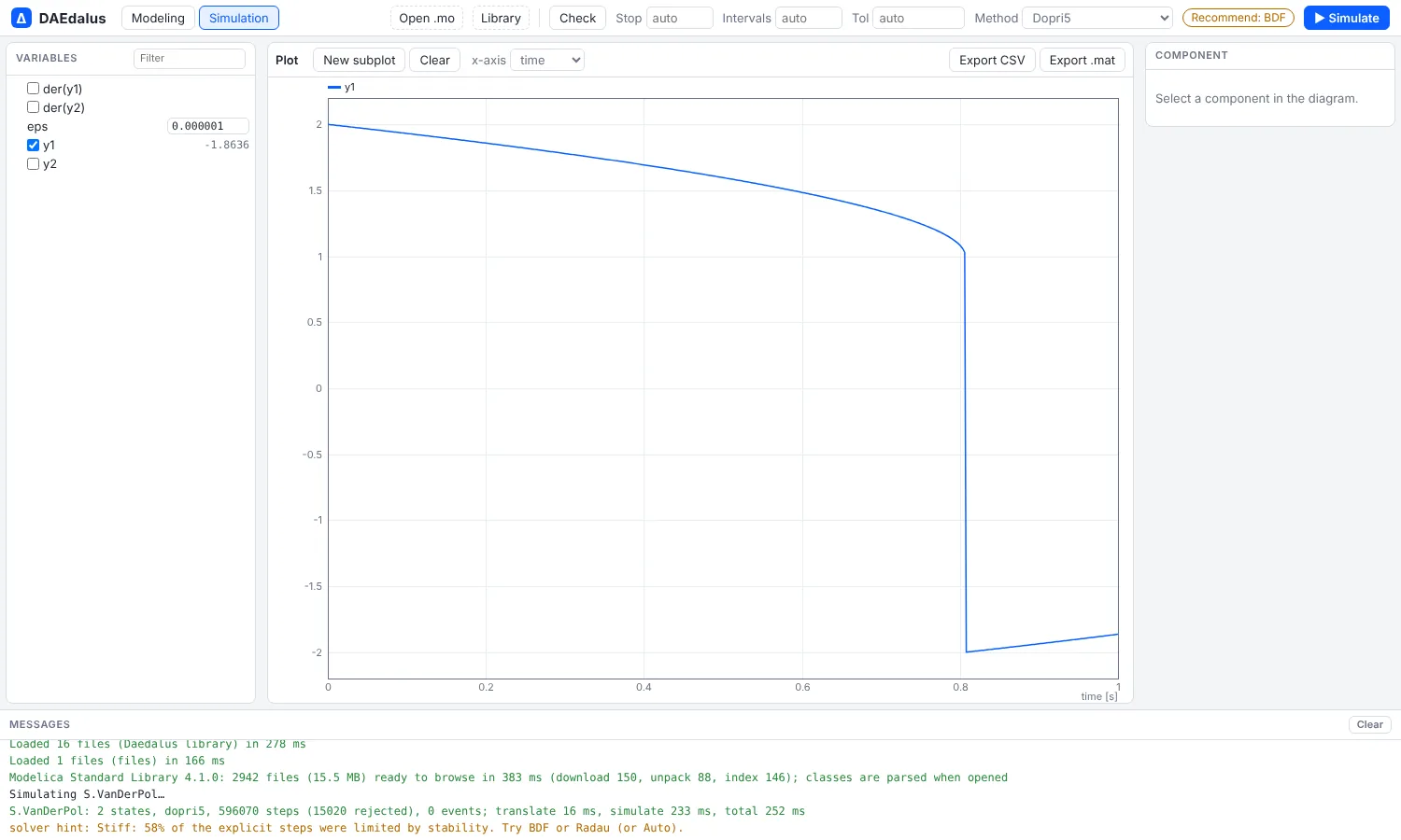
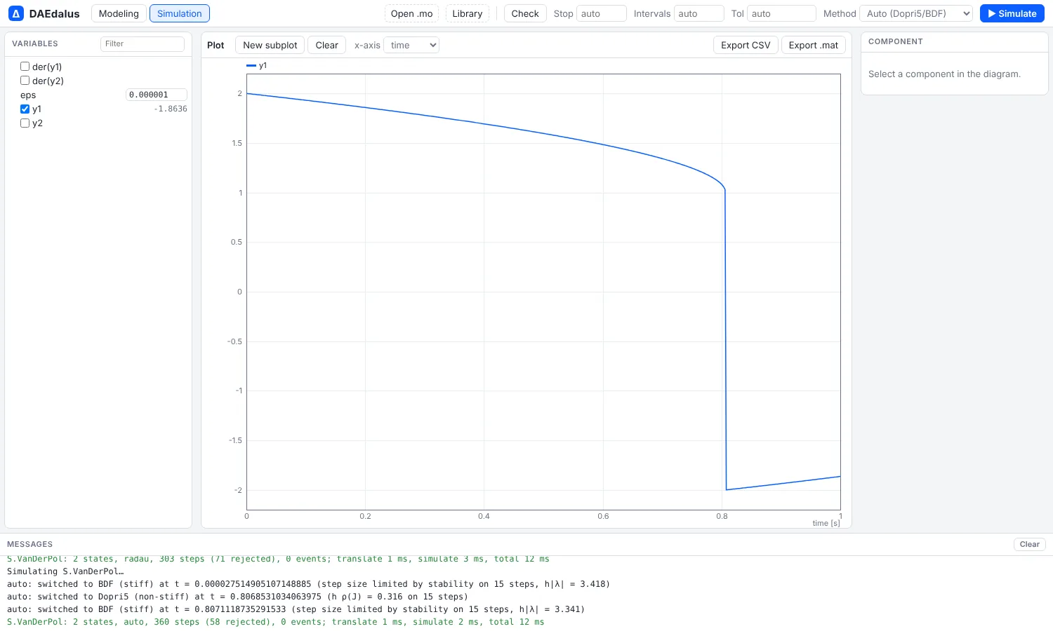
Clicking the chip selects the method for the next run. The hint uses only the run statistics. It does not do an eigenvalue analysis.
Tests
crates/daedalus-core/tests/solvers.rs with tests/models/stiff.mo:
- Robertson's kinetics at t = 40 and at t = 1e11, and Van der Pol with
mu = 1000 (
VDPOL, eps = 1e-6, t = 2), against the reference values of Hairer & Wanner's test set, for BDF, Radau, ESDIRK and Auto. - Prothero–Robinson with λ = -1e6 (stiff accuracy, and dense output between steps).
- A linear problem with an analytic solution: accuracy, dense output, and the
convergence order with the step forced by
max_step(observed 4.99 for Radau, 4.00 for ESDIRK). - A 60-cell heat equation (sparse Jacobian and sparse complex system) against its steady state.
- The bouncing ball with every new method (event times and heights).
- Auto switching both ways on a problem that is stiff only for
5 < t < 15. - Exact Jacobian against central differences (also through an algebraic loop), and BDF with exact and FD Jacobians giving the same results.
__Dymola_Algorithmnames and the experiment annotation.
solver_esdirk.rs checks the order conditions of the tableau (4 for the
solution, 3 for the embedded one).
Comparison
Best of three runs on a shared 4-core machine, so the times are approximate.
"f-evals" counts right-hand-side evaluations; with the exact Jacobian the
tangent passes are in parentheses after the Jacobian count. The bdf (before)
rows are the previous release with its finite-difference Jacobian. All runs use
each model's experiment tolerance unless stated.
| Model | Method | Steps | Rejected | f-evals | Jacobians (tape passes) | Sim time (ms) |
|---|---|---|---|---|---|---|
| QuarterCar.BumpComparison | bdf (before: FD Jacobian) | 1568 | 114 | 5534 | 109 | 27.0 |
| QuarterCar.BumpComparison | bdf (exact Jacobian) | 1568 | 114 | 4662 | 109 (872) | 27.1 |
| QuarterCar.BumpComparison | radau | 520 | 155 | 6572 | 318 (2544) | 29.2 |
| QuarterCar.BumpComparison | esdirk | 442 | 289 | 15128 | 150 (1200) | 35.2 |
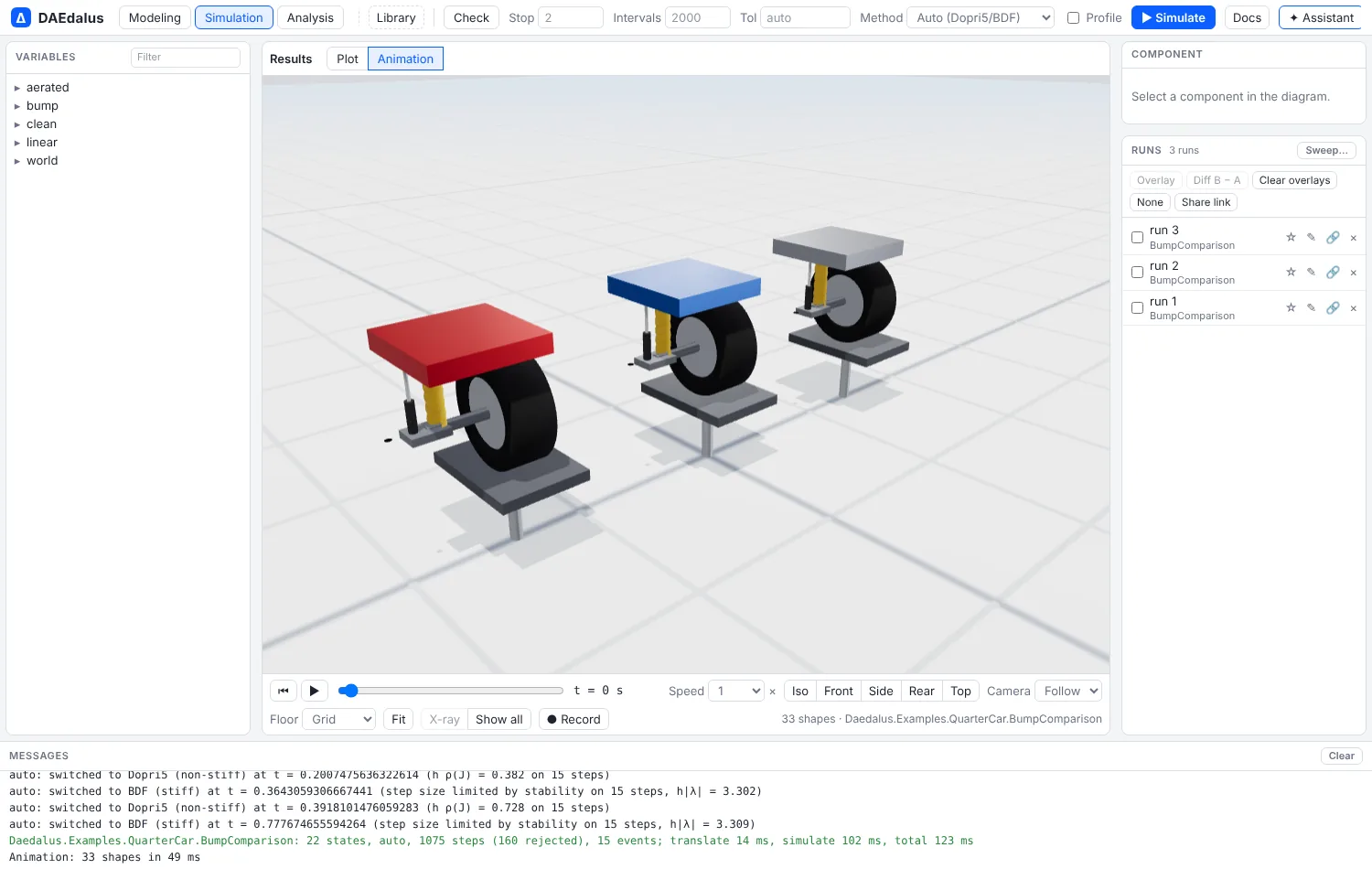
| QuarterCar.BumpComparison | auto | 1075 | 160 | 6533 | 27 (216) | 16.2 |
| TorqueConverter.Launch | bdf (before: FD Jacobian) | 644 | 80 | 1724 | 26 | 4.9 |
| TorqueConverter.Launch | bdf (exact Jacobian) | 644 | 80 | 1646 | 26 (78) | 4.7 |
| TorqueConverter.Launch | radau | 216 | 84 | 2354 | 71 (213) | 6.5 |
| TorqueConverter.Launch | esdirk | 157 | 149 | 5193 | 32 (96) | 8.0 |
| TorqueConverter.Launch | auto | 282 | 78 | 1563 | 8 (24) | 3.9 |
| LandingGear.SinkRates | bdf (before: FD Jacobian) | 913 | 42 | 2704 | 27 | 4.7 |
| LandingGear.SinkRates | bdf (exact Jacobian) | 913 | 42 | 2596 | 27 (108) | 4.9 |
| LandingGear.SinkRates | radau | 328 | 63 | 3315 | 135 (540) | 8.3 |
| LandingGear.SinkRates | esdirk | 274 | 85 | 7991 | 28 (112) | 18.5 |
| LandingGear.SinkRates | auto | 420 | 43 | 2742 | 1 (4) | 4.1 |
| VehicleEfficiency.UDDSEnergy | bdf (before: FD Jacobian) | 30618 | 4200 | 78671 | 1322 | 168.9 |
| VehicleEfficiency.UDDSEnergy | bdf (exact Jacobian) | 30617 | 4208 | 73398 | 1324 (5296) | 184.6 |
| VehicleEfficiency.UDDSEnergy | radau | 10718 | 5099 | 107536 | 3008 (12032) | 264.5 |
| VehicleEfficiency.UDDSEnergy | esdirk | 8365 | 8211 | 222833 | 1303 (5212) | 335.5 |
| VehicleEfficiency.UDDSEnergy | auto | 11035 | 3178 | 83802 | 34 (136) | 159.6 |
| Van der Pol mu=1000 (tol 1e-6) | bdf (before: FD Jacobian) | 1152 | 44 | 3772 | 60 | 0.7 |
| Van der Pol mu=1000 (tol 1e-6) | bdf (exact Jacobian) | 1152 | 44 | 3652 | 60 (120) | 0.7 |
| Van der Pol mu=1000 (tol 1e-6) | radau | 593 | 142 | 6949 | 197 (394) | 0.7 |
| Van der Pol mu=1000 (tol 1e-6) | esdirk | 632 | 201 | 21065 | 37 (74) | 1.1 |
| Van der Pol mu=1000 (tol 1e-6) | auto | 674 | 109 | 3708 | 60 (120) | 0.5 |
| Robertson to 1e5 (tol 1e-8) | bdf (before: FD Jacobian) | 429 | 1 | 1389 | 13 | 0.3 |
| Robertson to 1e5 (tol 1e-8) | bdf (exact Jacobian) | 427 | 1 | 1338 | 14 (42) | 0.4 |
| Robertson to 1e5 (tol 1e-8) | radau | 198 | 0 | 1638 | 40 (120) | 0.3 |
| Robertson to 1e5 (tol 1e-8) | esdirk | 124 | 92 | 3336 | 59 (177) | 0.3 |
| Robertson to 1e5 (tol 1e-8) | auto | 423 | 7 | 1455 | 12 (36) | 0.3 |
Notes:
- The exact Jacobian leaves the BDF step sequence essentially unchanged and
saves the right-hand-side evaluations of the differences. On the Daedalus
examples, BDF with the exact Jacobian and the previous BDF agree with a
1e-10 reference run equally well (the same worst state error on each of the
six examples checked).
--jacobian fdreproduces the previous step counts exactly. - Radau takes 2–3 times fewer steps than BDF. Each step costs more (three stages and a complex factorization), so it pays off on very stiff problems at tight tolerances rather than on these event-heavy examples.
- ESDIRK takes the fewest steps but needs more Newton iterations per step on strongly nonlinear problems (Van der Pol).
- Auto is the fastest on the Daedalus examples: they are stiff only in parts (hydraulic transients, contact), and Dopri5 is cheap in between.
Modelica Standard Library sweep
daedalus test-library msl -m Modelica --jobs 3 --timeout 60 over the 534
example models of MSL 4.1.0 (the bundle the workbench loads), each method at
the experiment tolerances:
| Method | Pass |
|---|---|
| bdf, previous release (FD Jacobian) | 471 |
| bdf, exact Jacobian | 471 |
| radau | 473 |
| auto | 471 |
- bdf, exact vs previous. One model is gained
(
Fluid.Examples.TraceSubstances.RoomCO2WithControls) and one is lost (Fluid.Examples.Tanks.TanksWithOverflow: event chatter at tolerance 1e-6. It passes with--jacobian fd, at other tolerances, and with radau, esdirk and auto). - radau passes seven models that BDF fails (
SimpleTriacCircuit,IMC_YDarc,Dimmer_RL,SoftStarter,SMEE_LoadDump,RobotR3.OneAxis,TanksWithOverflow). It fails or times out on some that BDF passes (DemoPowerSupplyWithBuffer,PolyphaseRectifier,ChopperStepDown_RL,HBridge,RoomCO2WithControls). - auto passes
TanksWithOverflowand failsDemoPowerSupplyWithBuffer: the model's back-current assertion fires during a Dopri5 phase. Models where Dopri5 cannot start (hysteresis tables, the heat exchanger) fall back to BDF at once.