Linearization

daedalus linearize computes the linear state-space model of a Modelica model around an operating point:

der(x) = A x + B u
     y = C x + D u

• x are the states DAEdalus selected (after index reduction, so dummy-derivative states are included);
• u are the model's top-level Real inputs, held at their start values (0 without one) while simulating to the point;
• y are its top-level Real outputs.

This is what Dymola's linearizeModel and OpenModelica's linearize do, and --format mo writes the same linearized_model that OpenModelica writes, so existing scripts can read it.

#Exact matrices

The matrices are exact, not finite differences. DAEdalus runs the compiled tape in forward mode once per state and input, and differentiates algebraic loops implicitly through their symbolic Jacobians, so a model with nonlinear loops linearizes as precisely as an explicit one. --jacobian fd uses central differences instead, as a cross-check.

#Example: a pendulum after one second

model Pendulum "nonlinear pendulum with a torque input"
  parameter Real L = 1;
  parameter Real g = 9.81;
  parameter Real d = 0.2;
  input Real tau;
  output Real angle;
  output Real height;
  Real phi(start = 0.5, fixed = true);
  Real w(start = 0, fixed = true);
equation
  der(phi) = w;
  L^2*der(w) = -g*L*sin(phi) - d*w + tau;
  angle = phi;
  height = -L*cos(phi);
end Pendulum;

daedalus linearize crates/daedalus-core/tests/models/linearize.mo -m Lin.Pendulum --at 1

linearization of Lin.Pendulum at t = 1
  jacobians: exact (forward-mode differentiation of the tape)

states (2):
  x[1] = phi  (-4.503617e-1)
  x[2] = w  (-7.710435e-2)

inputs (1):
  u[1] = tau  (0.000000e0)

outputs (2):
  y[1] = angle  (-4.503617e-1)
  y[2] = height  (-9.002897e-1)

A (2 x 2):
  [   0.000000e0    1.000000e0]
  [  -8.831842e0  -2.000000e-1]

B (2 x 1):
  [   0.000000e0]
  [   1.000000e0]

C (2 x 2):
  [   1.000000e0    0.000000e0]
  [ -4.352912e-1    0.000000e0]

D (2 x 1):
  [   0.000000e0]
  [   0.000000e0]

eigenvalues of A:
  -1.000000e-1 - 2.970159e0i
  -1.000000e-1 + 2.970159e0i

At t = 1 the pendulum swings through φ = −0.45 rad, so A[2,1] is −g·cos(φ)/L and the height output's sensitivity C[2,1] is sin(φ). The eigenvalues give a damped natural frequency of 2.97 rad/s.

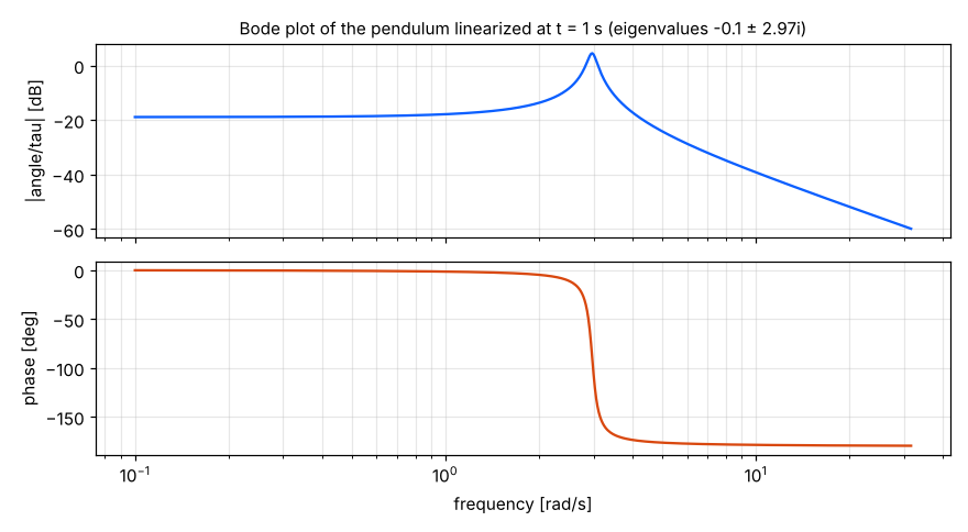
--format json writes the same matrices, names, operating point and eigenvalues as JSON, which makes a Bode plot a few lines of NumPy:

#OpenModelica-style output

daedalus linearize model.mo -m Lin.Pendulum --at 1 --format mo -o linearized_model.mo

model linearized_model "Lin.Pendulum"
  parameter Integer n = 2 "number of states";
  parameter Integer m = 1 "number of inputs";
  parameter Integer p = 2 "number of outputs";
  parameter Real x0[n] = {-0.4503617488561356, -0.07710435328579941};
  parameter Real u0[m] = {0};
  parameter Real y0[p] = {-0.4503617488561356, -0.9002896951544261};
  parameter Real dx0[n] = {-0.07710435328579941, 4.285627948331383} "der(x) at the linearization point";

  parameter Real A[n, n] =
	[0, 1;
	-8.83184190946492, -0.2];
  ...
  Real x[n](start=x0);
  input Real u[m](start=u0);
  output Real y[p];

  Real 'x_phi' = x[1];
  Real 'x_w' = x[2];
  Real 'u_tau' = u[1];
  Real 'y_angle' = y[1];
  Real 'y_height' = y[2];
equation
  der(x) = A * (x - x0) + B * (u - u0) + dx0;
  y = y0 + C * (x - x0) + D * (u - u0);
end linearized_model;

The model is written in affine form around the point, so it reproduces the nonlinear model's trajectory near it even away from an equilibrium (dx0 is not zero here). It is a plain Modelica model: daedalus check linearized_model.mo -m linearized_model translates it, and CI does exactly that on every pull request.

#Options

The CasADi export offers the same linearization from Python, as m.jacobians(), with the algebraic variables eliminated.